
I heard about Broadcasting for the first time in Lesson 9 of Jeremy Howard’s Introduction to Machine Learning for Coders. Jeremy went on and on about how important Broadcasting was…
The most important programming concept taught in this course and possibly the most important programming concept you will ever need to build machine learning algorithms.
Very few people in DataScience or Machine Learning community understand broadcasting.
If you get good at Broadcasting, you will have this super useful skill that very very few people have.
These wise words should be enough to pull you through to the end of the article.
Two tensors must have the same shape in order to perform element-wise operations on them and arithmetic operations are element-wise operations. Arithmetic operations on tensors with scalar values can be done in two ways:
- Using symbolic operations
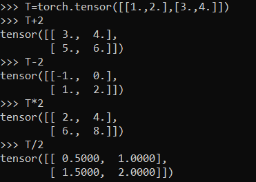
- Using built in tensor object methods
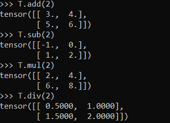
Both of these options work the same. We can see that in both cases, the scalar, is applied to each element with the corresponding arithmetic operation. Math here seems fine but these examples break the rule that element-wise operations operate on tensors of the same shape. Scalars are Rank-0 tensors, which means they have no shape, and our tensor T is a rank-2 tensor of shape 2 x 2. So how does this fit in? Let’s break it down.
The first solution that comes intuitively is that the operation is simply using the single scalar value and operating on each element within the tensor. This logic kind of works however, it’s a bit misleading and it breaks down in more general situations where we’re not using a scalar. To think about these operations differently, we need to introduce the concept of tensor broadcasting or broadcasting.

From Numpy documentation:
The term broadcasting describes how numpy treats arrays with different shapes during arithmetic operations. Subject to certain constraints, the smaller array is “broadcast” across the larger array so that they have compatible shapes. Broadcasting provides a means of vectorizing array operations so that looping occurs in C instead of Python. It does this without making needless copies of data and usually leads to efficient algorithm implementations.
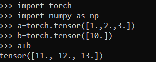
We can think of the scalar b being stretched during the arithmetic operation into an array with the same shape as a. The new elements in b are simply copies of the original scalar. The stretching analogy is only conceptual. NumPy is smart enough to use the original scalar value without actually making copies, so that broadcasting operations are as memory and computationally efficient as possible.
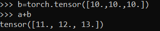
Another example of interaction between a vector and a tensor :
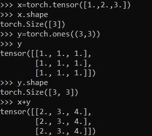
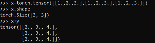
The element wise addition takes place as if x was broadcasted as follows to match the dimensions of y
Try wrapping your head around this trickier example :
.PNG)
Got your answer??
Is this your answer? 👇
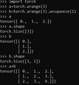
Just as before we stretched or broadcasted one tensor to match the shape of the other, here we’ve stretched both a and b to match a common shape, and the result is a two-dimensional array! The geometry of these examples is visualized in the following figure (Credits: Jake VanderPlas) :
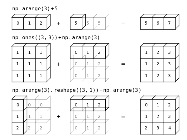
The light boxes represent the broadcasted values: again, this extra memory is not actually allocated in the course of the operation, but it can be useful conceptually to imagine that it is.
Step 1: Determining if the tensors are compatible
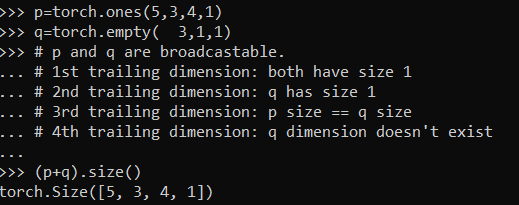
When operating on two arrays, Pytorch compares their shapes element-wise. It starts with the trailing(left most) dimensions, and works its way forward. Two dimensions are compatible when :
- they are equal, or
- one of them is 1
If these conditions are not met, an exception is thrown, indicating that the arrays have incompatible shapes.
Step 2: Determining the shape of the resulting tensor
If two tensors x, y are “broadcastable”, the resulting tensor size is calculated as follows:
- If the number of dimensions of x and y are not equal, prepend 1 to the dimensions of the tensor with fewer dimensions to make them equal length.
- Then, for each dimension size, the resulting dimension size is the max of the sizes of x and y along that dimension.
Rules of Broadcasting
- Rule 0: Each tensor has at least one dimension(trivial)
-
Rule 1: If the two arrays differ in their number of dimensions, the shape of the one with fewer dimensions is padded with ones on its leading (left) side.
-
Rule 2: If the shape of the two arrays does not match in any dimension, the array with shape equal to 1 in that dimension is stretched to match the other shape.
-
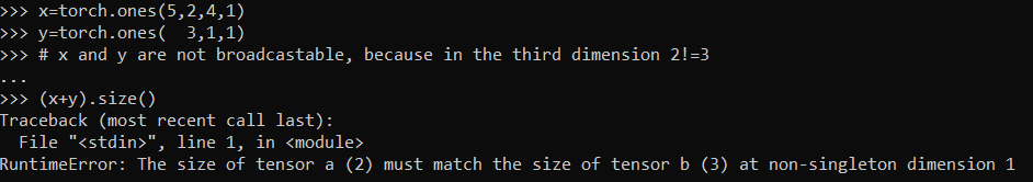
Rule 3: If in any dimension the sizes disagree and neither is equal to 1, an error is raised.
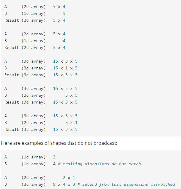
Here are a few tensors to truly make sense of these “rules”.
From Numpy Documentation:
This is the last piece of understanding how “tensors flow” in Pytorch. We all know that addition is commutative, x added to y is same as y added to x. Then why does Pytorch’s inplace addition function(add followed by an _) do this ? 👇
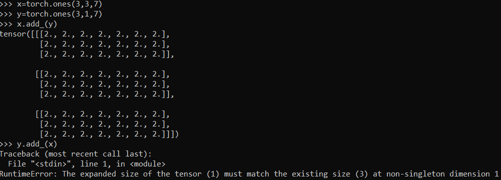
In-place operations do not allow the in-place tensor(x in first case and y in second case) to change shape as a result of the broadcast. Now we know why the inplace addition operation broke in the second case[tensor y was broadcasted to (3,3,7)].